Quickstart Guide

This is a step-by-step guide that aims to demonstrate two of the most typical use cases:

• computation of the auto-correlation function on regular-spaced data from standard DDM experiments performed with a single camera, and

• computation of the cross-correlation function on irregular-spaced data from the cross-DDM experiments using multiple-tau algorithm and real-time analysis.

For this guide you do not need the actual data because we will construct a sample video. We will be simulating a set of spherical particles undergoing 2D Brownian. Simulation is performed on-the-fly with the Brownian motion simulator that is included with this package. In real world experiments you will have to stream the videos either directly from the cameras with the library of your choice, or read data files from the disk. This package does not provide the tools for reading the data, so it is up to the user to provide the link between the image readout and the correlation computation functions. You can use imageio or any other tool for loading recorded videos.

To proceed, you can copy-paste the examples below in your python shell. Or, if you have the package source downloaded and examples/ folder in your sys.path, open the source files under each of the plots in this document and run them in your favorite python development environment.

Video processing

We will start with some basic video processing functions and explain the data types used in the package. We will demonstrate the use on single-camera video first, and then show how to process dual-camera experiment on irregular-spaced data as demonstrated in the Cross-DDM paper.

Video data type

In cddm.video there are a few video processing functions that were designed to work on iterables of multi-frame data. This way you can process the data without reading it into the memory. It is also possible to analyze live videos without first writing the videos to disk.

Video data is an iterable object with tuple elements, where each tuple holds a set of numpy arrays (frames). A single-camera video is an iterator over a single-frame tuples. A dual-camera video iterates over dual frame data (two numpy arrays). To clarify, a valid dual-frame out-of-memory video can be constructed using python generator expressions, e.g. for random noise dual-frame video of length 1024 you can do:

>>> import numpy as np
>>> video = ((np.random.rand(512,512), np.random.rand(512,512)) for i in range(1024))

Check python documentation on generator expressions if you are unfamiliar with the above expression. Here, video is an iterable object that can be used to acquire images frame-by-frame without reading the whole data into memory, making it possible to analyze long videos. A valid single-frame video is therefore:

>>> video = ((np.random.rand(512,512),) for i in range(1024))

Notice the trailing comma to indicate a tuple of length 1. The above random noise video is a multi-frame video holding only a single array in each of the elements of the video iterable object. Note that any iterable is valid, so you can work with lists, or tuples, or create any object of your own that support the iterator protocol.

Video simulator

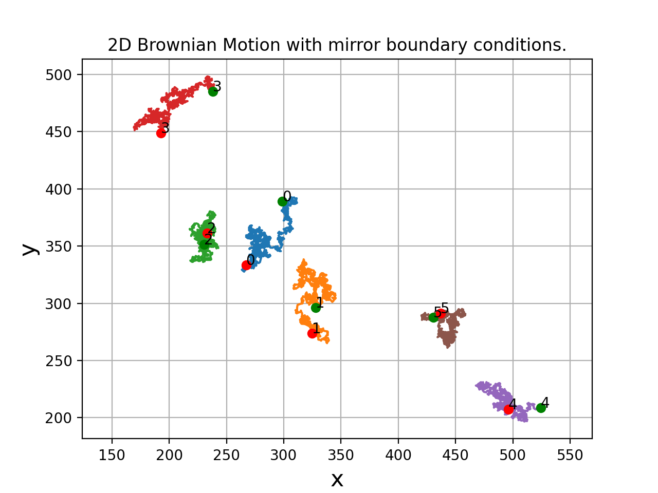
For testing, we will build a sample video of a simulated Brownian motion of 100 particles. We will construct a simulation area of shape (512+32,512+32) because we will later crop this to a shape of (512,512).

>>> from cddm.sim import plot_random_walk, seed
>>> seed(0) #sets numba and numpy seeds for random number generators
>>> plot_random_walk(count = 1024, particles = 6, shape = (512+32,512+32))

Fig. 1 2D random walk simulation of 6 particles. Green dots indicate start positions, red dots are the end positions of the particles. (Source code, png, hires.png, pdf)

We crop the simulated video in order to avoid mirroring of particles as they touch the boundary of the simulation size because of the mirror boundary conditions implied by the simulation procedure. This way we simulate the real-world boundary effects better and prevent the particles to reappear on the other side of the image when they leave the viewing area.

>>> from cddm.sim import simple_brownian_video, seed
>>> seed(0) #sets numba and numpy seeds for random number generators
>>> t = range(1024) #times at which to trigger the camera.
>>> video = simple_brownian_video(t, shape = (512+32,512+32),
...    delta = 2, dt = 1, particles = 100, background = 200,
...    intensity = 5, sigma = 3)

Here we have created a frame iterator of Brownian motion of spherical particles viewed with a camera that is triggered with a constant frame rate (standard DDM experiment). Time t goes in units of time step defined with parameter \(\delta t = 1\), specified by the simulator. The delta parameter is the mean step size (if dt=1) in units of pixel size. It is related to the diffusion constant D by the relation \(\delta = \sqrt{2D}\). Particles are of Gaussian shape with sigma = 3, have peak intensity of 5, background intensity (static illumination) is 200. Images are of uint8 dtype.

Showing video

You may want to inspect and play videos. Video player is implemented in the module viewer using matplotlib. It is not meant to be a real-time player, but it allows you to inspect the video before you begin the correlation analysis. In order to inspect the video, we will first load the video into memory (though you are not required to):

>>> from cddm.video import load
>>> video = load(video, 1024) #allows you to display progress bar
>>> video = list(video) #or this
>>> video = tuple(video) #or this

Note

For playing the video you are not required to load the data into memory. By doing so, it allows you to inspect the video back and forth, otherwise we can only iterate step by step in the forward direction with the viewer.VideoViewer.

Now we can inspect the video:

>>> from cddm.viewer import VideoViewer
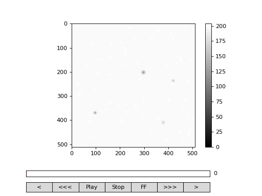
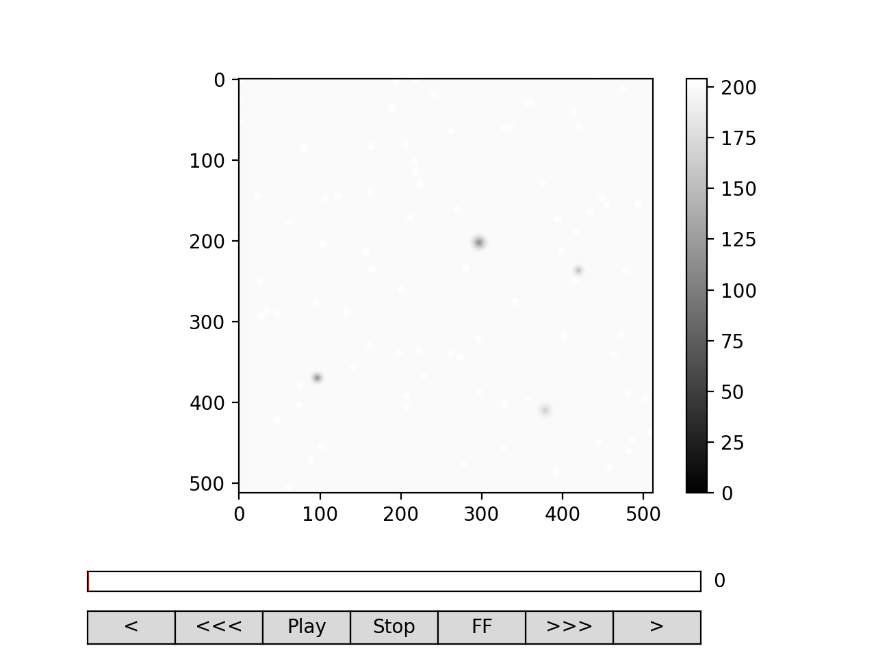
>>> viewer = VideoViewer(video, count = 1024, vmin = 0, cmap = "gray")
>>> viewer.show()

Fig. 2 viewer.VideoViewer can be used to visualize the video (in memory or out-of-memory). (Source code, png, hires.png, pdf)

See also

For real-time video visualizations see Live video.

Cropping

You may want to crop the data before processing. Cropping is done using python slice objects, or simply, by specifying the range of values for slicing. For instance to perform slicing of frames (numpy arrays) like frame[0:512,0:512] do:

>>> from cddm.video import crop
>>> video = crop(video, roi = ((0,512), (0, 512)))

Under the hood, the crop function performs array slicing using slice object generated from the provided roi values. See video.crop() for details. You can crop to any shape, however, you must be aware that in reciprocal space, non-rectangular data has a different unit step size, so care must be made in the interpretation of wave vector values of the FFTs performed on non-rectangular data.

Windowing

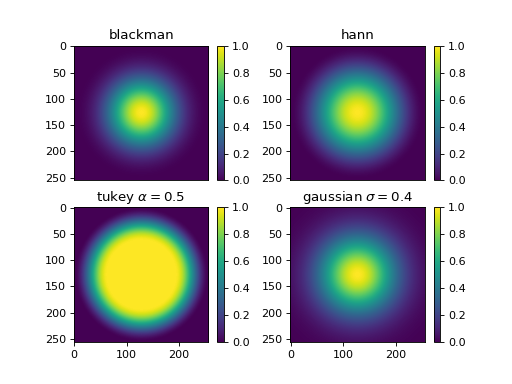
In FFT processing, it is common to apply a window function before the computation of FFT in order to reduce FFT leakage. In cross-DDM it also helps to reduce the camera misalignment error. In window there are four 2D windowing functions that you can use.

>>> from cddm.window import plot_windows
>>> plot_windows()

Fig. 3 There are four 2D windowing functions that you can use. (Source code, png, hires.png, pdf)

After you have cropped the data you can apply the window. First create the window with the shape of the frame shape of (512,512). For blackman filtering, do:

>>> from cddm.window import blackman
>>> window = blackman((512,512))

In order to multiply each frame of our video with this window function we must create another video-like object. This video must be of the same length and same frame shape as the video we wish to process. Use generator expression mechanism or tuple/list creation mechanism to build this video-like object:

>>> window_video = ((window,),)* 1024
>>> video = multiply(video, window_video)

Again, notice the trailing commas.

Performing FFT

The next thing is to compute the FFT of each frame in the video and to generate a FFT video. The FFT video is a an iterable with a multi-frame data, where each of the frames in the elements of the iterable holds FFT of the frames of the video. Because the input signal is real, there is no benefit in using the general FFT algorithm for complex data and to hold reference to all computed Fourier coefficients. Instead, it is better to compute or hold reference only for the first half of the coefficients using np.fft.rfft2, for instance, instead of np.fft.fft2. For this reason, the package provides a fft.rfft2() function that works on iterables, and there is no equivalent fft2 function.

Note

The underlying k-averaging and data visualization functions expect the fft data to be presented in half-space only. So if you make your own fft2 function, you must crop the data to half space!

Also, in DDM experiments there is usually a cutoff wavenumber above which there is no significant signal to process. To reduce the memory requirements and computational effort, it is therefore better to remove the computed coefficients that will not be used in the analysis. You can do this using:

>>> from cddm.fft import rfft2
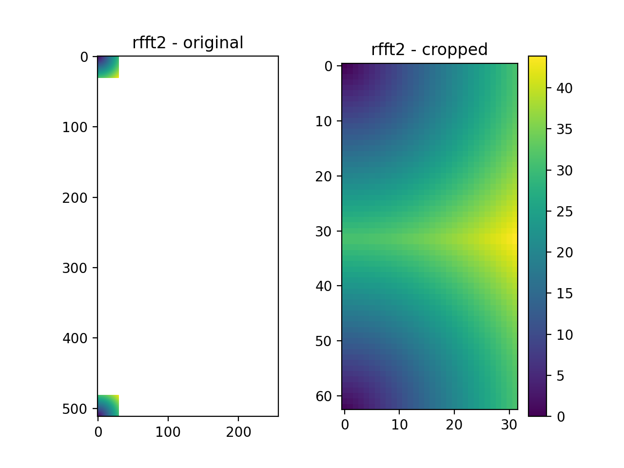
>>> fft = rfft2(video, kimax = 31, kjmax = 31)

Here, the resulting fft object is of the same video data type. We have used two arguments kimax and kjmax for cropping. The result of this cropping is a video of FFTs, where the shape of each frame (in our case it is a single frame of the multi-frame data type) is \((2*k_{imax}+1, k_{jmax} +1)\). As in the uncropped rfft2, the zero wave vector is found at[0,0], element [31,31] are for the largest wave vector k = (31,31), element [-1,0] == [62,0] of the cropped fft is the Fourier coefficient of k = (-1,0). The original rfft2 frame shape in our case is (512,257), and therefore the max possible k value for our dataset is \(k_{max} = (\pm 257,257)\). With kimax and kjmax we have reduced the computation size for the correlation function calculation from (512*257) to (63*32) different k vectors, which significantly improves the speed and lowers the memory requirements.

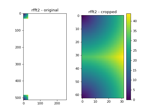
Fig. 4 We take only a small subset of the original k-values. (Source code, png, hires.png, pdf)

See also

Data masking demonstrates how to use more advanced k-masking features.

Bakground removal

It is important that background removal is performed at some stage, either before the computation of the correlation or after, using proper normalization procedure. If you can obtain the (possibly time-dependent) background frame from a separate experiment you can subtract the frames either in real space (done before calling rfft2):

>>> from cddm.video import subtract
>>> background = np.zeros((512,512)) # zero background
>>> background_video = ((background,),) * 1024
>>> video = subtract(video, background_video)

or in reciprocal space:

>>> background = np.zeros((63,32)) + 0j # zero background
>>> background_fft = ((background,),) * 1024
>>> fft = subtract(fft, background_fft)

However, most of the times it is not possible to acquire a good estimator of the background image. The algorithm allows you to remove the background within the normalization procedure, so it is not necessary to fully remove the background prior to the calculation of the correlation function.

Until now, none of the processing has yet took place because all processing functions that were applied have not yet been executed. The execution of the video processing function takes place in real-time when we start the iteration over the frames, e.g. when we calculate the correlation function. If you need to inspect the results of the video processing you have to load the calculation results in memory. To load the results of the processing into memory, to inspect the data you can do

>>> fft = list(fft)
>>> fft = tuple(fft) #or this

Note

For the iterative versions of the correlation algorithms you do not need to load the data into memory.

Converting to/from arrays

You can convert multi-frame video to numpy arrays and numpy arrays to video with video.asarrays() and video.fromarrays(). We are currently working with one-element (single camera) video. To load the video from previous examples into numpy array do:

>>> from cddm.video import fromarrays, asarrays
>>> fft_array, = asarrays(fft, count = 1024)

Notice the trailing comma. Function video.asarrays() returns a tuple of numpy arrays. The length of the tuple depends on the number of frames in the multi-frame video object. In our case, we have a single frame, so a single array is returned. To construct a single-frame video object, do

>>> fft_iter = fromarrays((fft_array,))

Again, notice the trailing comma, indicating a single-frame video. A dual-frame video iterator requires two equally-shaped numpy arrays in the data tuple.

Auto-correlation

Now that our video has been cropped, windowed, normalized, Fourier transformed, we can start calculating the correlation function. There are a few ways to calculate the correlation function (or image structure function) with the cddm package. Here we will do a standard auto-correlation analysis first, then we will do the multiple-tau approach, as this is the most efficient way to simultaneously obtain small delay and large delay time data. There is an in-memory version of the algorithm, working on numpy arrays and an out-of-memory version working on the video data iterable objects that we defined above in our previous examples.

Linear analysis

For standard regular time-spaced data analysis, if you need to calculate all delay times that are accessible from the measured data, you will have to use the calculation methods from core and you will have to load the data into numpy array first, as shown in Converting to/from arrays. Then do:

>>> from cddm.core import acorr, normalize, stats
>>> acorr_data = acorr(fft_array)

Here acorr_data is a raw correlation data that still needs to be normalized. When computing with default arguments, it is a tuple of length 5, but it can also be of length 4 if different parameters are used. As a user, you do not need to know the details of this data type. If you are curious, thought, it will be defined in detail later in Representation modes. What you need to know at this stage is that the first element of the correlation data tuple is the actual correlation data, the second element is the count data.

>>> corr = acorr_data[0]
>>> count = acorr_data[1]

Here the shape of the data are

>>> corr.shape == (63,32,1024) and count.shape == (1024,)
True

For most simple normalization (assuming background subtraction has been performed prior to the calculation of the correlation function) you could do

>>> normalized_data = corr/count

However, for more complex, background removing normalizations you will normalize the data using core.normalize(). Details about the normalization types will be covered in Norm & Method. For default normalization, you have to provide the mean and pixel variance data of the original fft data. You can use core.stats() to compute these:

>>> bg, var = stats(fft_array)
>>> lin_data = normalize(acorr_data, bg, var, scale = True)

We used the scale option to scale the data between 0 and 1 (normalize with variance). lin_data is the normalized autocorrelation data that you can plot and analyze. It is a numpy array, the shape of the data depends on the input fft_array shape. In our case it is

>>> lin_data.shape == (63,32,1024)
True

You can inspect the data with viewer.DataViewer

>>> from cddm.viewer import DataViewer
>>> viewer = DataViewer(shape = (512,512)) # shape not needed here
>>> viewer.set_data(lin_data)
>>> viewer.set_mask(k=25, angle = 0, sector = 30)
True

Note

For rectangular-shaped video frames, the unit size in k-space is identical in both dimensions, and you do not need to provide the shape argument, however, for non-rectangular data, the step size in k-space is not identical. The shape argument is used to calculate unit steps for proper k-visualization and averaging.

Now we can plot the data:

>>> viewer.plot()
>>> viewer.show()

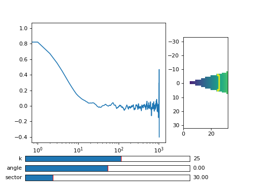
Fig. 5 viewer.DataViewer can be used to visualize the normalized correlation data. With sliders you can select the size of the wave vector k, angle of the wave vector with respect to the horizontal axis, and averaging sector. The resulting correlation function that is shown on the left subplot is a mean value of the computed correlation functions at the wave vectors that are marked in the right subplot. (Source code, png, hires.png, pdf)

See also

There is also viewer.CorrViewer that you can use to inspect raw correlation data.

Log averaging

Usually, when correlation function is exponentially decaying it is best to have data log spaced. You can average the linear data at larger time delays and do:

>>> t, log_data = log_average(lin_data)

Here, t is the log-spaced time delay array, log_data is the log-spaced correlation data. The first two axes are for the i- and j-indices of the wave vector k = (ki,kj), the last axis of y is the time-dependent correlation data. Therefore, to plot the computed correlation function as a function of time do:

>>> import matplotlib.pyplot as plt
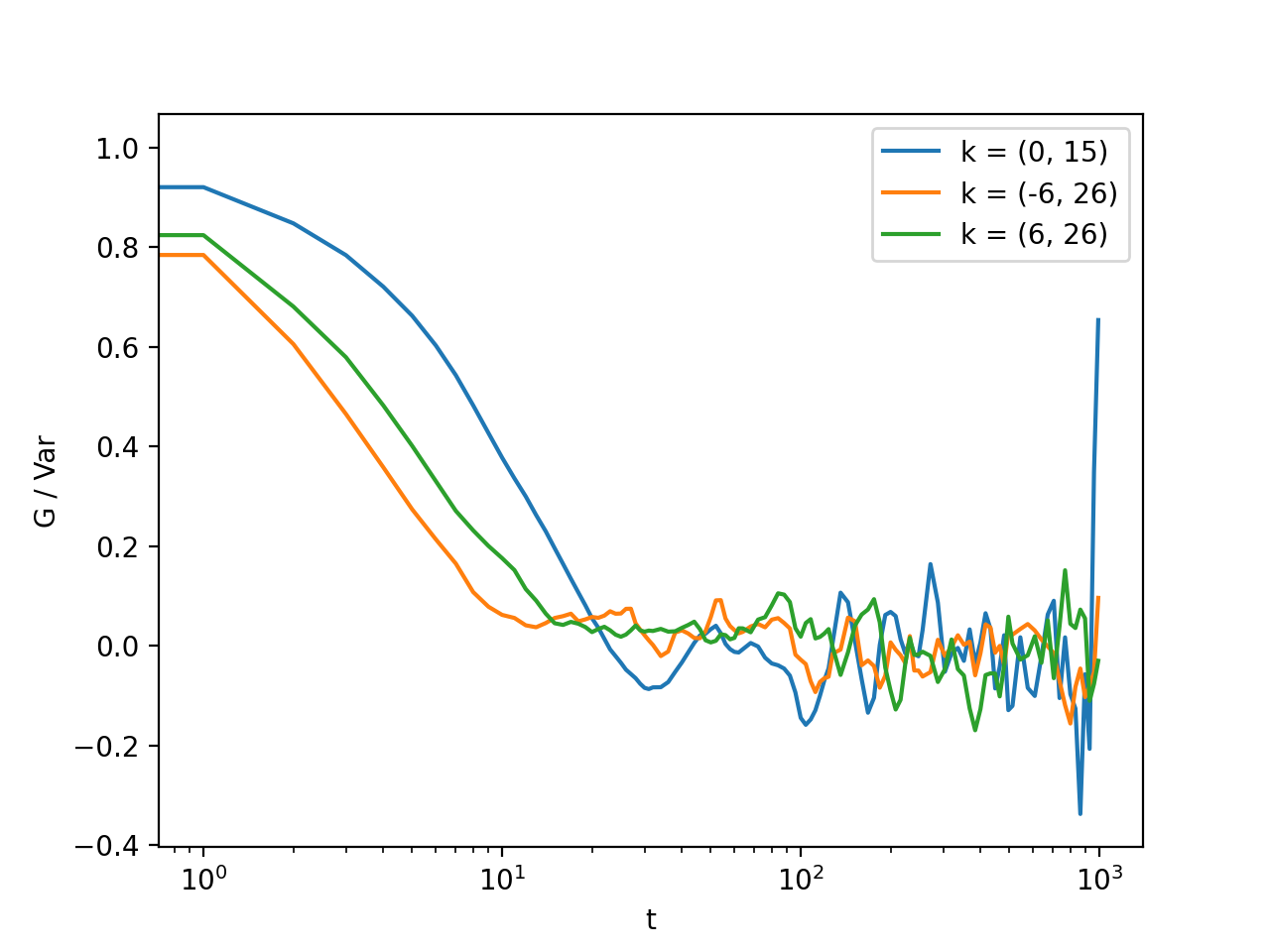
>>> for (i,j) in ((0,15),(-6,26), (6,26)):
...     ax = plt.semilogx(t,log_data[i,j], label =  "k = ({}, {})".format(i,j))
>>> legend = plt.legend()
>>> text = plt.xlabel("time delay")
>>> text = plt.ylabel("G/Var")
>>> plt.show()

Fig. 6 Log-spaced data example. In the first axis, you can access negative coefficients. (Source code, png, hires.png, pdf)

That is it, you are done! Now you can save the data in the numpy data format for later use:

>>> np.save("t.npy", t)
>>> np.save("data.npy", log_data)

If you wish to analyze the data with some other tool (Mathematica, Origin) you will have to google for help on how to import the numpy binary data. Another option is to save as text files. But you have to do it index by index. For instance, to save the (4,8) k-value data, you can do:

>>> i, j = 4, 8
>>> np.savetxt("data_{}_{}.txt".format(i,j), log_data[i,j])

Now you can use your favorite tool for data analysis and fitting. But, most probably you will want to do some k-averaging. This will be covered in Data analysis, so keep reading.

Multitau analysis

Instead of doing the linear analysis and log averaging, you can use the multiple-tau algorithm to achieve similar results. In module multitau there is a multitau version of the core.acorr() called multitau.acorr_multi() that you can use. Here we will work with the iterative version multitau.iacorr_multi() which works on data iterators.

Note

There is also an iterative version of the core.acorr() called core.iacorr() that you can use for linear analysis on limited delay time range. See API, and extra examples in the source.

To perform multiple tau correlation analysis, you have to provide the FFT iterator and define how many frames to analyze

>>> from cddm.multitau import iacorr_multi
>>> data, bg, var = iacorr_multi(fft, count = 1024)

The output of the multitau.iacorr_multi(), by default, returns a data tuple with a structure that will be defined shortly, and two additional arrays (mean pixel value array and pixel variance array) that are needed for normalization. First, let us inspect the data using viewer.MultitauViewer

>>> from cddm.viewer import MultitauViewer
>>> viewer = MultitauViewer(scale = True, shape = (512,512))
>>> viewer.set_data(data, bg, var)
>>> viewer.set_mask(k = 25, angle = 0, sector = 30)
True

We used the scale = True option to normalize data to pixel variance value, which results in scaling the data between (0,1).

Note

For rectangular-shaped video frames, the unit size in k-space is identical in both dimensions, and you do not need to provide the shape argument, however, for non-rectangular data, the step size in k-space is not identical. The shape argument is used to calculate unit steps for proper k-visualization and averaging.

Plot the data:

>>> viewer.plot()
>>> viewer.show()

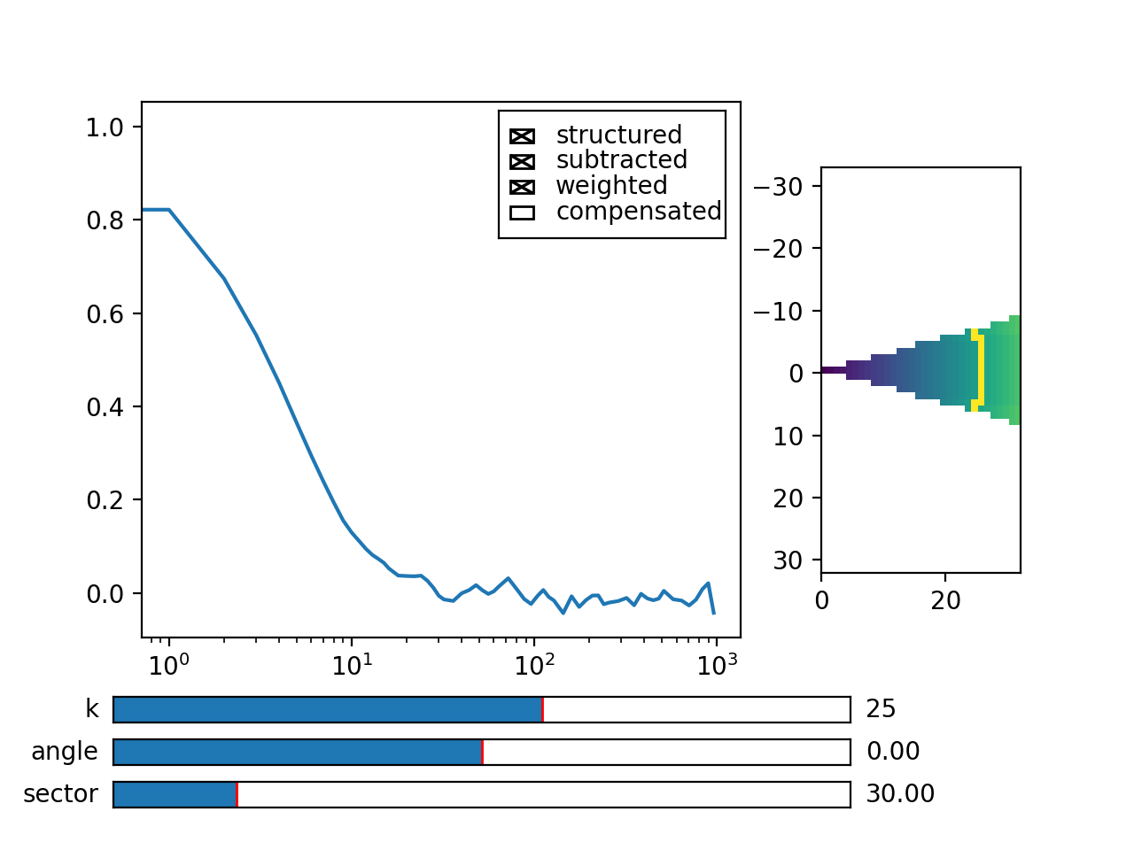
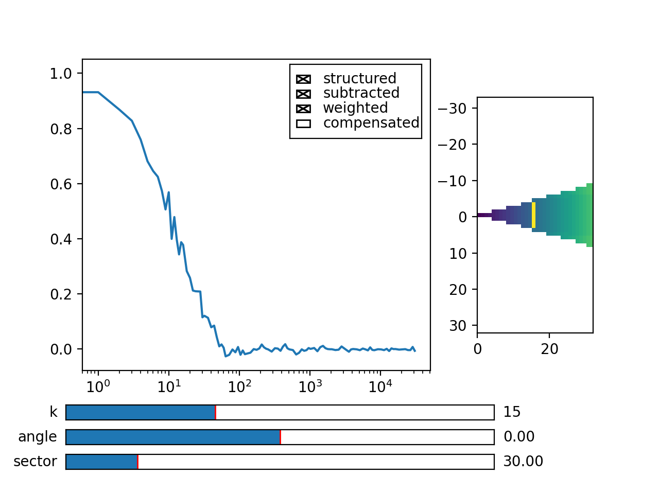
Fig. 7 viewer.MultitauViewer can be used to visualize the correlation data. With sliders you can select the size of the wave vector k, angle of the wave vector with respect to the horizontal axis, and averaging sector. The resulting correlation function that is shown on the left subplot is a mean value of the computed correlation functions at the wave vectors that are marked in the right subplot. (Source code, png, hires.png, pdf)

Multitau data

The multitau correlation data itself resides in a tuple of two elements

>>> lin_data, multi_level = data

Both lin_data and multi_data are the correlation data tuples as defined in Linear analysis. The actual correlation data is the first element

>>> corr_lin = lin_data[0]
>>> corr_multi = multi_level[0]

The second element is the count data, which count the number of realizations of a given time delay, which is needed for the most basic normalization.

>>> count_lin = lin_data[1]
>>> count_multi = multi_level[1]

Here the shape of the data are

>>> corr_lin.shape == (63,32,16) and count_lin.shape == (16,)
True
>>> corr_multi.shape == (6,63,32,16) and count_multi.shape == (6,16)
True

The lin_data is the zero-th level of the multiple-tau data, while multi_level is the rest of the multi-level data. By default the size of each level in multilevel data is 16, so we have 16 time delays for each level, and there are 63 x 32 unique k values. The multi_level part of the data has 6 levels, the length of corr_multi varies, and depends on the length of the video. The rest of the data elements of the lin_data and multi_data are time-dependent sum of the signal squared and time-dependent sum of signal for each of the levels, which are needed for more advanced normalization. You do not need to know the exact structure, because you will not work with the raw correlation data, but you will use the provided normalization functions to convert this raw data into meaningful normalized correlation function.

Merging multitau data

We can compare the results obtained from the multiple tau approach with the linear analysis and log averaging from the previous example. Fist we normalize the data:

>>> from cddm.multitau import normalize_multi, log_merge
>>> lin_data, multi_level = normalize_multi(data, bg, var, scale = True)

Here, lin_data and multi_level are normalized correlation data (numpy arrays). One final step is to merge the multi_level part with the linear part into one continuous log-spaced data.

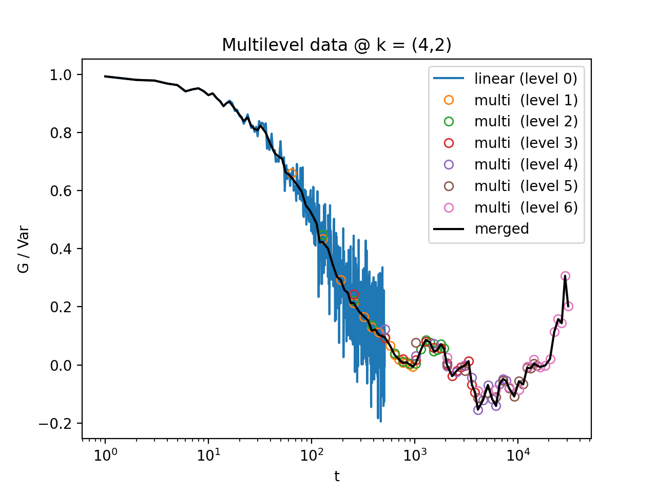
>>> x, y = log_merge(lin_data, multi_level)

Here, x is the log-spaced time delay array, y is the merged correlation data.

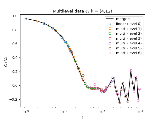
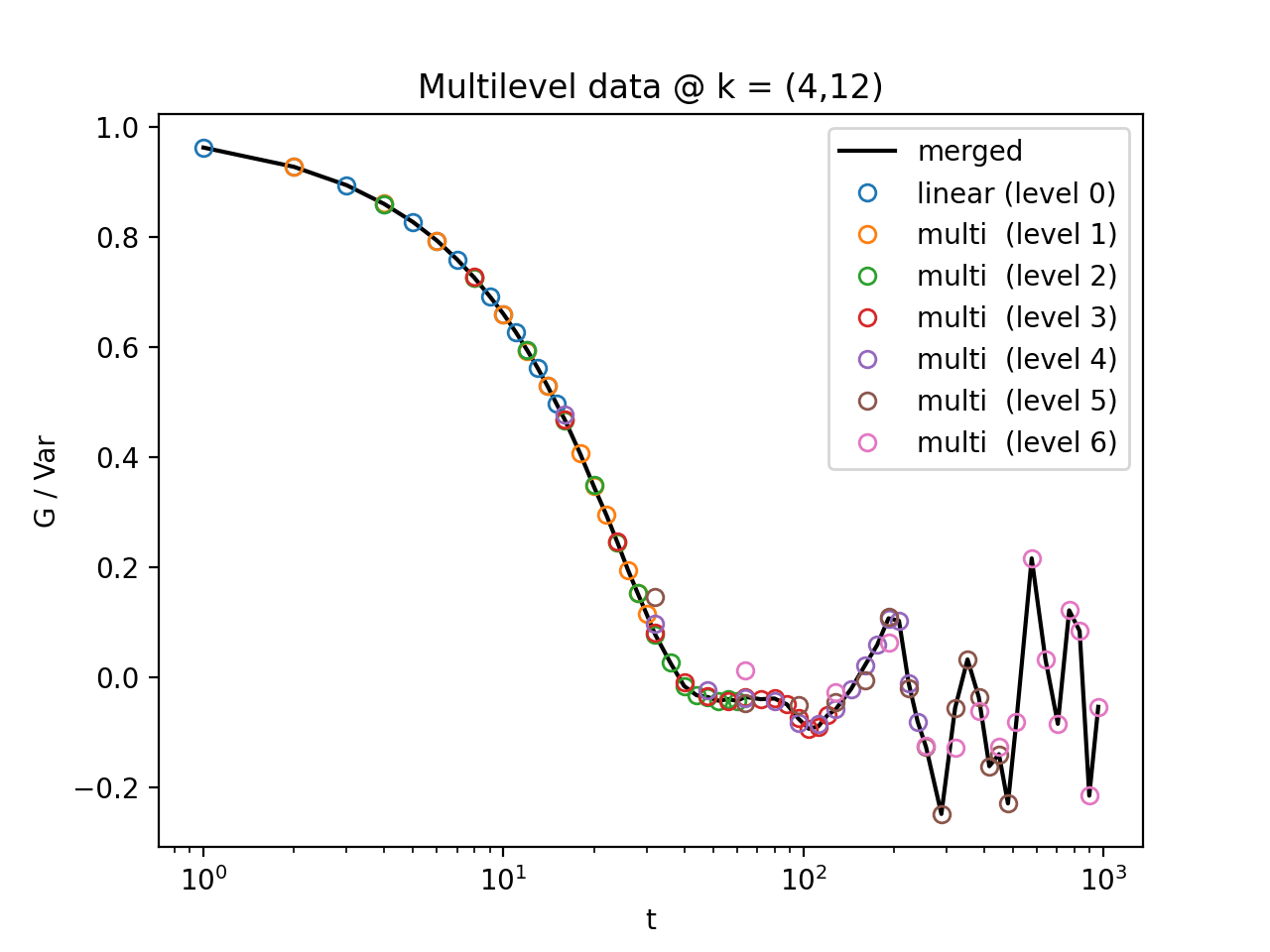
Fig. 8 All levels of the multilevel data and the merged data (black). (Source code, png, hires.png, pdf)

We can compare the log merged results with the log averaged results:

>>> for (i,j) in ((4,12),(-6,16)):
...    l = plt.semilogx(t,log_data[i,j], label =  "averaged k = ({}, {})".format(i,j) )
...    l = plt.semilogx(x,y[i,j], label =  "multitau k = ({}, {})".format(i,j) )
>>> text = plt.xlabel("t")
>>> text = plt.ylabel("G / Var")
>>> legend = plt.legend()
>>> plt.show()

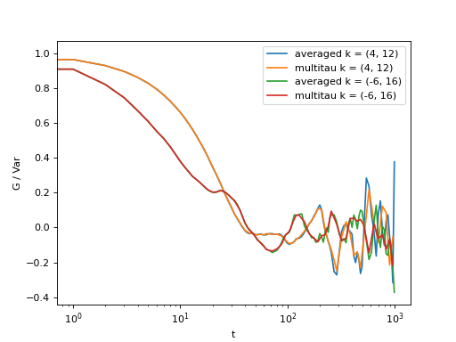
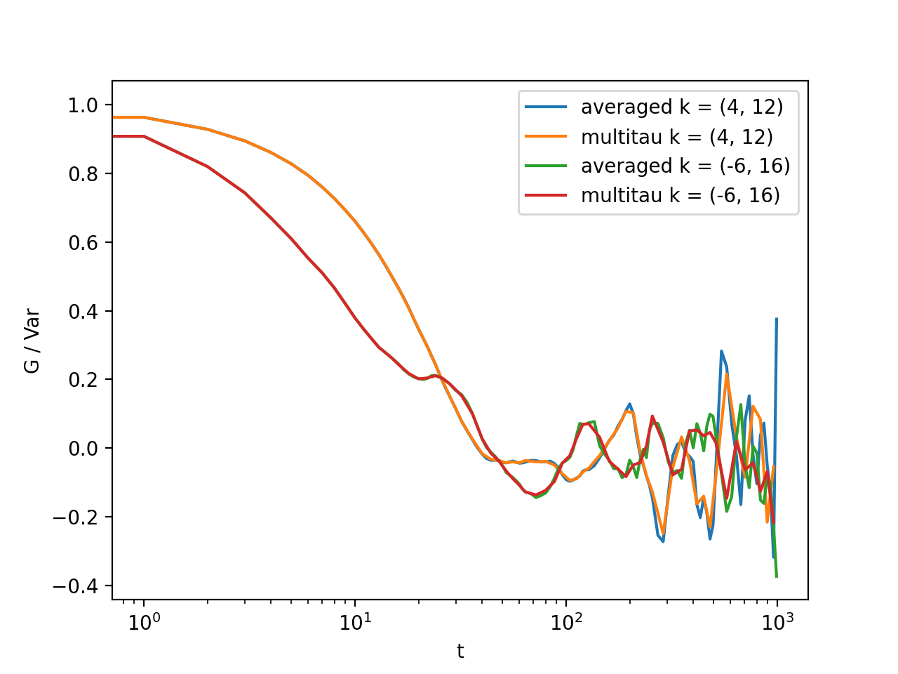
Fig. 9 Data obtained using multiple tau algorithm is comparable to the log averaged linear data. Slight discrepancy comes from the difference between the averaging performed with the multitau.log_average() and the effective averaging of the multiple tau algorithm. (Source code, png, hires.png, pdf)

As you can see, both yield similar results. Slight discrepancy comes from the difference between the averaging performed with the multitau.log_average() and the effective averaging implied by the multiple tau algorithm.

Cross-correlation

Cross correlation can be made on two different (or equal) sources of data. Normalized results of the cross-correlation performed on two equal datasets are identical to the result obtained form the auto-correlation function (slight discrepancy is due to data-dependent numerical error of the method), e.g.:

>>> from cddm.core import ccorr
>>> bg, var = stats(fft_array, fft_array)
>>> ccorr_data = ccorr(fft_array, fft_array)
>>> acorr_data = acorr(fft_array)
>>> lin_data_cross = normalize(ccorr_data, bg, var, scale = True)
>>> lin_data_auto  = normalize(acorr_data, bg, var, scale = True)
>>> np.allclose(lin_data_auto, lin_data_cross, atol = 1e-4) #almost the same.
True

Irregular-spaced data analysis

To compute the cross-correlation of randomly-triggered dual-camera videos, as demonstrated in the paper, the computation is basically the same. Cross-correlation with irregular spaced data using multiple tau algorithm can be done in the following way. Import the tools needed:

>>> from cddm.viewer import MultitauViewer
>>> from cddm.video import multiply,  crop
>>> from cddm.window import blackman
>>> from cddm.fft import rfft2
>>> from cddm.multitau import iccorr_multi, normalize_multi, log_merge
>>> from cddm.sim import simple_brownian_video, create_random_times1

Now, set up random time sequence and video of the simulated cross-DDM experiment

>>> t1, t2 = create_random_times1(1024,n = 16)
>>> video = simple_brownian_video(t1,t2, shape = (512+32,512+32))
>>> video = crop(video, roi = ((0,512), (0,512)))

Here the parameter n defines the random triggering scheme as explained in the paper. The effective period of the trigger is in our case \(period = 2 * n\). We will apply some dust particles to each frame in order to simulate different static background on the two cameras. If your working directory is in the examples folder you can load dust images:

>>> dust1 = plt.imread('data/dust1.png')[...,0] #float normalized to (0,1)
>>> dust2 = plt.imread('data/dust2.png')[...,0]
>>> dust = ((dust1,dust2),)*nframes
>>> video = multiply(video, dust)

To view the two videos we can use the VideoViewer

>>> video = list(video)
>>> viewer1 = VideoViewer(video, count = 1024, id = 0, vmin = 0, cmap = "gray")
>>> viewer1.show()
>>> viewer2 = VideoViewer(video, count = 1024, id = 1, vmin = 0, cmap = "gray")
>>> viewer2.show()

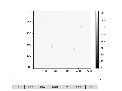
Fig. 10 (png, hires.png, pdf) Dust particles on the two cameras are different, which result in different background frames. (Source code)

Fig. 11 (png, hires.png, pdf) Dust particles on the two cameras are different, which result in different background frames. (Source code)

Intensity jitter compensation

In cross-DDM, if you use a pulsed light source, and if you face issues with the stability of the intensity of the light source (intensity jitter), you can normalize each frame with respect to the mean value of the frame. This way you can avoid flickering effects, but you will introduce additional noise because of the randomness of the scattering process (randomness of the mean scattering value).

>>> from cddm.video import normalize_video
>>> video = normalize_video(video)

Pre-process the video and perform FFT

>>> window = blackman((512,512))
>>> window_video = ((window,window),)*1024
>>> video = multiply(video, window_video)
>>> fft = rfft2(video, kimax =31, kjmax = 31)

Optionally, you can normalize for flickering effects in fft space, instead of normaliing in real space.

>>> from cddm.fft import normalize_fft
>>> fft = normalize_fft(fft)
>>> fft = list(fft) #not really needed if you are going to process fft only once

Again, do this only if you have problems with the stability of the light source.

Live analysis

To show live view of the computed correlation function during data iteration, we can pass the viewer as an argument to multitau.iccorr_multi():

>>> viewer = MultitauViewer(scale = True, shape = (512,512))
>>> viewer.k = 15 #initial mask parameters,
>>> viewer.sector = 30
>>> data, bg, var = iccorr_multi(fft, t1, t2, period = 32, viewer  = viewer)

Note

For rectangular-shaped video frames, the unit size in k-space is identical in both dimensions, and you do not need to provide the shape argument, however, for non-rectangular data, the step size in k-space is not identical. The shape argument is used to calculate unit steps for proper k-visualization and averaging.

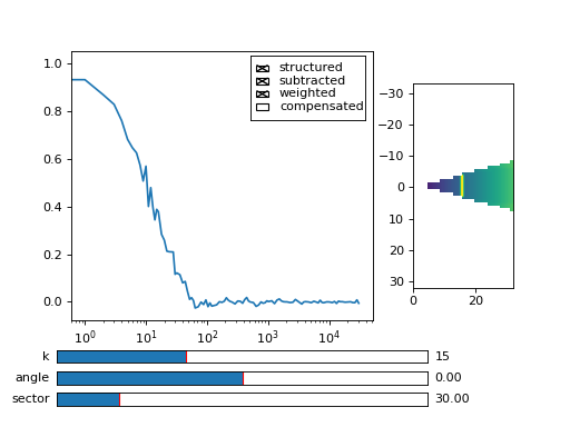
Fig. 12 You can see the computation in real-time. The rate of refresh can be tuned with the viewer_interval argument. (Source code, png, hires.png, pdf)

Note the period argument. You must provide the correct effective period of the random triggering of the cross-ddm experiment. The bg and var are now tuples of arrays of mean pixel and pixel variances of each of the two videos.

Warning

Data will not be merged and processed correctly if the period argument does not match the period used in the experiment. Care must be taken not to mix up this parameter or t1 and t2 time sequences, as there is no easy way to determine the period from t1, and t2 parameters alone.

Note

Live data view uses matplotlib for visualization, which is slow in rendering. It will significantly reduce the computational power. In numerically intensive experiments (high frame rate and large k-space) you will probably have to disable real-time rendering.

Merging multitau data

As for the auto correlation on regular spaced data, the irregular spaced data must be normalized and merged.

>>> from cddm.multitau import normalize_multi, log_merge
>>> lin_data, multi_level = normalize_multi(data, bg, var, scale = True)

Here, lin_data and multi_level are normalized correlation data (numpy arrays). One final step is to merge the multi_level part with the linear part into one continuous log-spaced data.

>>> x, y = log_merge(lin_data, multi_level)

Here, x is the log-spaced time delay array, y is the merged correlation data. Raw data and the merged results is shown below.

Fig. 13 All levels of the multilevel data and the merged data (black). (Source code, png, hires.png, pdf)

Data analysis

Now that we have calculated the correlation function, it is time to do one final step: we need to analyze the data. First, to improve the statistics, it is wise to perform some sort of k-averaging over neighboring wave vectors. We have already used the MultitauViewer to visualize the data and do the averaging, so we can use the viewer to obtain the k-averaged data:

>>> ok = viewer.set_mask(k = 10, angle = 0, sector = 30)
>>> if ok: # if mask is not empty, if valid k-value exist in the mask
...    k = viewer.get_k() #average value of the size of the wave vector
...    x, y = viewer.get_data() #averaged data

You have to do this index by index. Another way is to work with the normalized data and use the map.k_select() generator function, like:

>>> from cddm.map import k_select
>>> fast, slow = normalize_multi(data, bg, var, scale = True)
>>> x,y = log_merge(fast, slow)
>>> k_data = k_select(y, angle = 0, sector = 30, shape = (512,512))

Here, k_data is an iterator of (k_avg, data_avg) elements, where k_avg is the mean size of the wavevector and data_avg is the averaged data. You can save the averaged data to txt files. Example below will save all non-zero data at all k-values within the selection criteria defined above:

>>> for (k_avg, data_avg) in k_data:
...    np.savetxt("data_{}.txt".format(k_avg), data_avg)

Note

For rectangular-shaped video frames, the unit size in k-space is identical in both dimensions, and you do not need to provide the shape argument, however, for non-rectangular data, the step size in k-space is not identical. The shape argument is used to calculate unit steps for proper k-visualization and averaging.

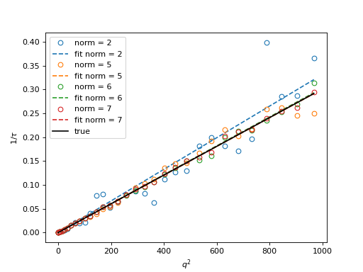
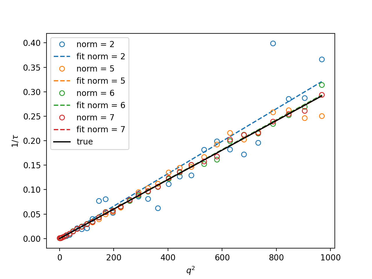
In the examples in this guide we were simulating Brownian motion of particles, so the correlation function decays exponentially. The obtained relaxation rate is proportional to the square of the wave vector, so we can obtain the diffusion constant and compare the results with the theoretical prediction. See the source of the plots below to perform k-averaging and fitting in python. The example below demonstrates how to fit data, that was normalized with different normalization modes (see next section for details on normalization modes).

Fig. 14 Results from the fitting of the cross-correlation function computed with multitau.iccorr_multi() using subtract_background = False option. For this example, the norm = 6 datapoint are closest to the theoretically predicted value shown in graph with the black line. (Source code, png, hires.png, pdf)

As can be seen, normalization with norm = 7 appears to work best with this data. norm = 7 normalization mode is the default mode used in the normalization procedure. It is a weighted normalization mode that works best on most data. It is computationally most complex, and there may be times when you will use different normalizations. These are explained in the next section.

Norm & Method

Correlation function can be computed and normalized with different normalization modes. This is controlled both in the computation functions, e.g. core.acorr() and in the normalize functions, e.g. core.normalize() with the norm flags. This works in combination with the method used in the calculation. Each of the computation functions accepts the method argument that controls the computation method. This way you can tune the accuracy and speed of the calculation of the correlation function. By now we have used the default values for the calculation methods and normalization modes, which work well for most data, but in some specific cases you might want to change these default settings.

In addition, the normalized data can be viewed in two different data representations, either with mode = ‘corr’ (the default representation), for standard correlation data representation, or mode = ‘diff’, for difference (or image structure function) representation of the data. These options are explained in this section.

The methods

When computing the correlation function there are three different methods to choose from:

• method = ‘corr’ for standard correlation \(C_k=\sum_i I_i I_{i+k}\) (good for multiple tau algorithm on irregular spaced data)

• method = ‘fft’ computes \(C_k=\sum_i I_i I_{i+k}\) through FFT (good for linear algorithm with regular spaced data)

• method = ‘diff’ for the differential algorithm \(D_k= \sum_i \left|I_i -I_{i+k}\right|^2\) (good for multiple tau algorithm on irregular spaced data with norm = 1)

There are no restrictions in norm selection if you use the first two methods, the differential method, however, support norm = 1 or norm = 3 in cross-correlation analysis and norm = 1 in auto-correlation analysis.

Norm flags

By default, computation and normalization is performed using

>>> from cddm.core import NORM_SUBTRACTED, NORM_WEIGHTED, NORM_STANDARD, NORM_STRUCTURED
>>> norm = NORM_SUBTRACTED | NORM_WEIGHTED
>>> norm == 7
True

There is a helper function, to build normalization flags:

>>> from cddm.core import norm_flags
>>> norm_flags(subtracted = True, weighted = True)
7

When calculation of the correlation function is performed with norm = NORM_SUBTRACTED | NORM_WEIGHTED or with norm = NORM_SUBTRACTED | NORM_STRUCTURED, a full calculation is performed. This way it is possible to normalize the computed data with the multitau.normalize() or multitau.normalize_multi() functions in six different ways.

Standard normalization

For standard (non-weighted) normalization do:

• standard : norm = NORM_STANDARD (norm = 1), supported methods: ‘corr’ and ‘fft’ here we remove the baseline error introduced by the non-zero background frame, which produces an offset in the correlation data. For this to work, you must provide the background data to the multitau.normalize_multi() or core.normalize().

• structured : norm = NORM_STRUCTURED (norm = 2), here we compensate the statistical error introduced at smaller delay times. Basically, we normalize the data as if we had calculated the cross-difference (structure) function instead of the cross-correlation. This requires one to calculate the delay-dependent squares of the intensities, so one extra channel, which slows down the computation when method = ‘corr’ or ‘fft’.

• subtracted standard : norm = NORM_STANDARD | NORM_SUBTRACTED ` (`norm = 5), supported methods: ‘corr’ and ‘fft’. Here we compensate for baseline error and for the linear error introduced by the not-known-in-advance background data. This requires one to track the delay-dependent sum of the data, so two extra channels.

• subtracted structured : norm = NORM_STRUCTURED | NORM_SUBTRACTED (norm = 6), which does both the subtracted and structured normalizations. Here, ‘diff’ method is supported only in cross-analysis and not in auto-analysis. This is the most complex computation mode, as there are three additional channels to track.

norm 2 or norm 6 data are better for low lag times, while norm 1 or norm 5 have less noise and a more stable baseline at larger lag times.

Note

Since V0.3.0 there is also an experimental implementation of a compensated normalization. Use the NORM_COMPENSATED flag in conjunction with NORM_STANDARD and NORM_STRUCTURED to use it. Currently this normalization scheme works well for linear data, but it should not be used in multitau algorithms. Also note that in previous versions, the structured normalization was termed compensated. The naming changed in V0.3.0 in order to be consistent with the compensated normalization scheme that was established for photon correlation analysis.

Weighted normalization

There are two weighted normalization modes that are supported only for calculation methods: ‘corr’ and ‘fft’. These are:

• weighted : norm = NORM_WEIGHTED (norm = 3). Performs weighted average of structured and standard normalized data. The weighting factor is to promote large delay data from standard data and short delay from structured data.

• subtracted weighted : norm = NORM_SUBTRACTED | NORM_WEIGHTED (norm = 7) Performs weighted average of subtracted structured and subtracted standard normalized data. The weighting factor is to promote large delay data from standard data and short delay from structured data.

To describe how these work internally, we will perform weighted normalization manually. First, data is normalized with structured (and background subtracted) and standard (and background subtracted) modes:

>>> lin_5, multi_5 = normalize_multi(data, bg, var, norm = 5, scale = True)
>>> lin_6, multi_6 = normalize_multi(data, bg, var, norm = 6, scale = True)

Then, correlation data estimator is calculated from the structured data. Denoising is applied, data is clipped between (0,1) because we have scaled the data. If data is not scaled, you can use the core.scale_factor() to compute the proper scaling factor. Data is shaped so that it is monotonously decreasing:

>>> from cddm.avg import denoise, decreasing
>>> x,y = log_merge(lin_6, multi_6)
>>> y = denoise(decreasing(np.clip(denoise(y),0,1)))

This way we have built a correlation data estimator that is then used to interpolate weighting array. For linear part of the data you can build this using.

>>> from cddm.avg import weight_from_data, weighted_sum, log_interpolate
>>> x_new = np.arange(lin_6.shape[-1])
>>> w = weight_from_data(y, pre_filter = False)
>>> w = log_interpolate(x_new, x, w)

Here we have used pre_filter = False option, because we have already filtered the data. With pre_filter=True same denoising is performed as in the example above. The calculated weight is for the standard data (norm = 5). The weight for the structured data is \(1 - w\). You can do the weighted sum:

>>> lin = weighted_sum(lin_5,lin_6, w)

For the multilevel part, the procedure is the same, except that the x coordinates for the interpolator are different. There is a helper function to build the x coordinates of the multilevel data:

>>> from cddm.multitau import t_multilevel
>>> x_new = t_multilevel(multi_6.shape, period = 32)
>>> w = weight_from_data(y, pre_filter = False)
>>> w = log_interpolate(x_new, x, w)
>>> multi = weighted_sum(multi_5,multi_6, w)

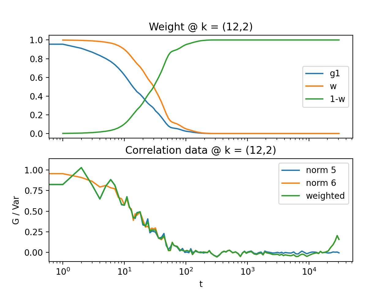
for details, see source code in the example below. The weights w`and `1 - w are for norm = 5 and norm = 6 data, respectively.

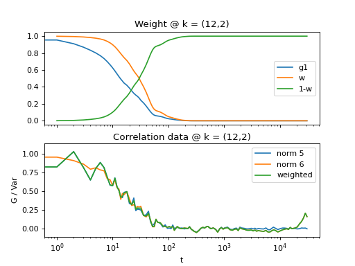
Fig. 15 Demonstrates how to perform weighted sum of norm = 6 and norm = 6 data. First, norm 6 data is taken as a first estimator, data is denoised and weights are calculated and a weighted sum of norm 6 and norm 5 data is performed. (Source code, png, hires.png, pdf)

Note that for the calculation of the correlation data with e.g. multitau.ccorr_multi(), norm = NORM_SUBTRACTED | NORM_WEIGHTED (norm = 6) is identical to norm = NORM_SUBTRACTED | NORM_STRUCTURED (norm = 5), and norm = NORM_WEIGHTED (norm = 3) is identical to norm = NORM_STRUCTURED (norm = 2). In the normalization, the results are different, as shown in graphs below.

Note

core.NORM_WEIGHTED is a shorthand for NORM_STANDARD|NORM_STRUCTURED

Instead of manually calculating the weights, you can use the norm argument and pass it to the normalize functions, like:

>>> i,j = 4,15
>>> for norm in (1,2,3,5,6,7):
...    fast, slow = normalize_multi(data, bg, var, norm = norm, scale = True)
...    x,y = log_merge(fast, slow)
...    ax = plt.semilogx(x,y[i,j], label =  "norm = {}".format(norm) )
>>> text = plt.xlabel("t")
>>> text = plt.ylabel("G / Var")
>>> legend = plt.legend()
>>> plt.show()

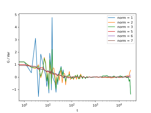
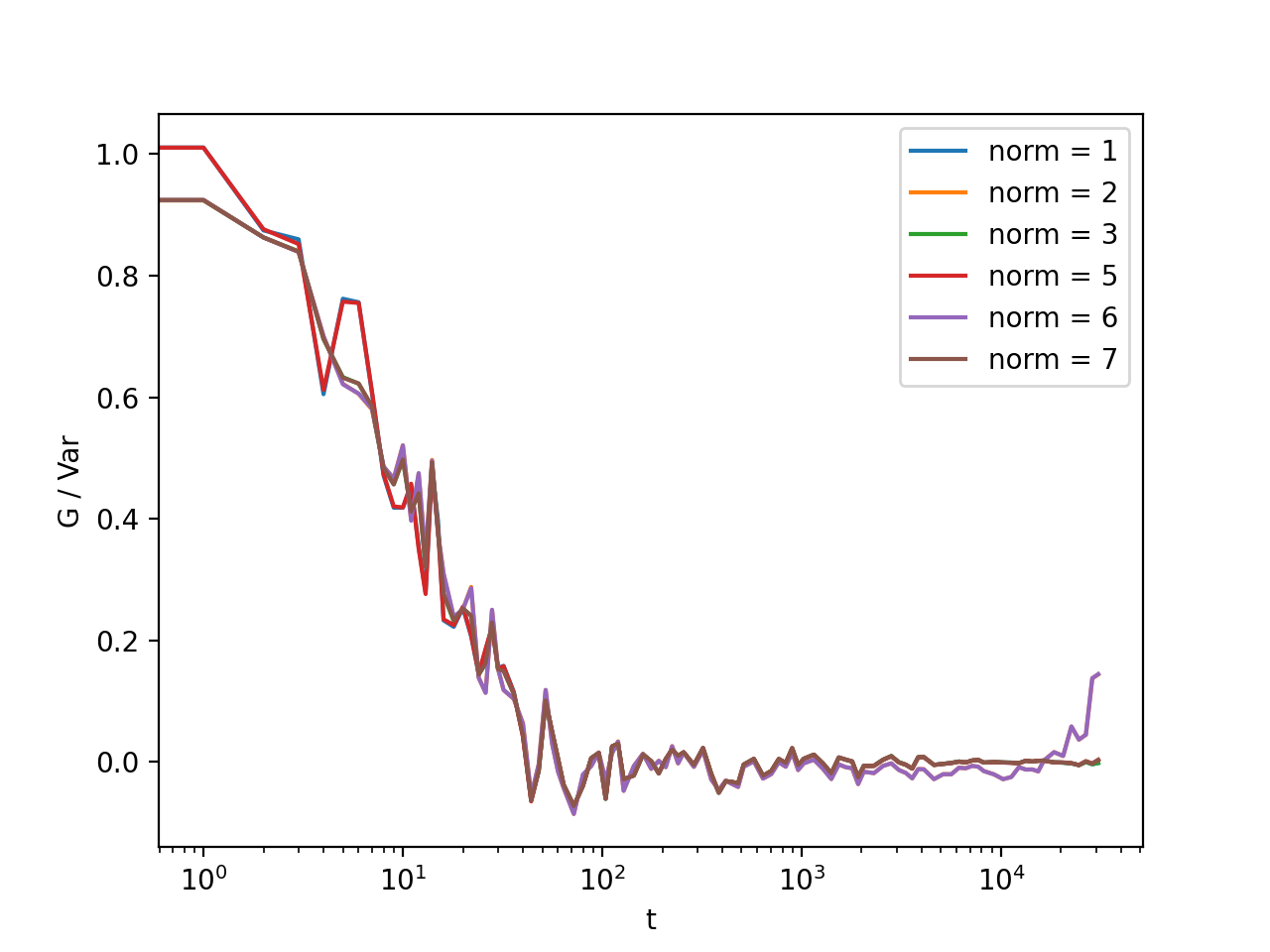
Fig. 16 Normalization mode 6 works best for small time delays, mode 5 works best for large delays and is more noisy at smaller delays. Mode 7 is weighted sums of mode 5 and 6 and have a lower noise in general. Mode 3 is weighted sums of mode 1 and 2. Here, the main contribution of the noise comes from the background, so it is important that background subtraction is performed. (Source code, png, hires.png, pdf)

Auto background removal

If you know which normalization mode you are going to use, you may reduce the computational effort in some cases. For instance, the main reason to use modes 5 and 6 (or 7) is to properly remove the two different background frames from both cameras. Usually, this background frame is not known until the experiment is finished, so the background subtraction is done after the calculation of the correlation function is performed. However, this requires that we track two extra channels that are measuring the delay-dependent data sum for each of the camera, or one additional channel that is measuring the delay-dependent sum of the squares of the data on both cameras. This significantly slows down the computation by a factor of 3 approximately.

One way to partially overcome this limitation is to use the auto_background option and to define a large enough chunk_size.

>>> data, bg, var = iccorr_multi(fft, t1, t2, period = 32, chunk_size = 128, auto_background = True)

This way we have forced the algorithm to work with chunks of data of length 128, and to take the first chunk of data to calculate the background frames that are then used to subtract from the input video. This way we get a reasonably good estimator of the background, which reduces the need to use the NORM_SUBTRACTED flag for the normalization as shown below.

>>> i,j = 4,15
>>> for norm in (1,2,3,5,6,7):
...    fast, slow = normalize_multi(data, bg, var, norm = norm, scale = True)
...    x,y = log_merge(fast, slow)
...    ax = plt.semilogx(x,y[i,j], label =  "norm = {}".format(norm) )
>>> text = plt.xlabel("t")
>>> text = plt.ylabel("G / Var")
>>> legend = plt.legend()
>>> plt.show()

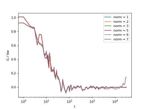
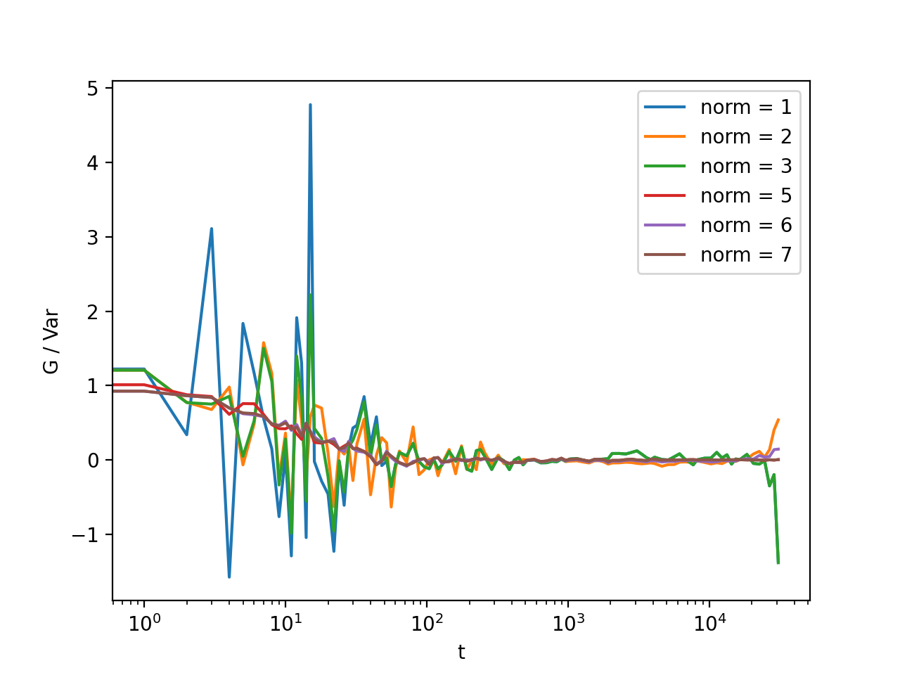
Fig. 17 Background frame has been succesfuly subtracted and there is no real benefit in using the NORM_SUBTRACTED flag (norm = 5 or norm = 6), and we can work with NORM_STANDARD (norm = 1) or NORM_STRUCTURED (norm = 2). (Source code, png, hires.png, pdf)

Note

If the background is properly subtracted before the calculation of the correlation function, the output of normalize functions with norm = 1 and norm = 5 are identical, and the output of normalize function with norm = 1 and norm = 3 are identical, and so the output of norm = 2 is identical to norm = 6. In the case above, background has not been fully subtracted, so there is still a small difference.

In some experiments, it may be sufficient to work with norm = 1, and you can work with:

>>> data, bg, var = iccorr_multi(fft, t1, t2, period = 32,
...         norm = NORM_STANDARD, chunk_size = 128, auto_background = True)

which will significantly improve the speed of computation, as there is no need to track the three extra channels. In case you do need the structured normalization, you can do:

>>> data, bg, var = iccorr_multi(fft, t1, t2, period = 32,
...         norm = NORM_STRUCTURED, chunk_size = 128, auto_background = True)

This will allow you to normalize either to standard or structured, but the computation is slower because of one extra channels that needs to be calculated.

Note

In non-ergodic systems auto-background subtraction may not work sufficiently well, so you are encouraged to work with norm = 3 or 7 during the calculation, and later decide on the normalization procedure. You should calculate with norm < 3 only if you need to gain the speed, or to reduce the memory requirements.

Representation modes

The cddm package defines two different correlation data representation modes. Either mode = ‘corr’ for correlation mode or mode = ‘diff’ for image difference mode (typically used in standard DDM experiments). Both modes are equivalent and we can convert from the difference mode to the correlation mode. However, the computation with different methods yield different intermediate results. It is after we call the core.normalize() that data become equivalent. This is demonstrated below.

Auto/Cross-correlation can be computed using direct calculation method=’corr’, or using Circular-Convolution theorem by means of FFT transform method=’fft’. For regular-spaced data and standard linear analysis , the ‘fft’ algorithm is usually the fastest, and is used by default. The output of ccorr and acorr functions depend on the method used. For method=’corr’ and method=’fft’, the output of acorr is

>>> acorr_data = acorr(fft_array, method = "fft") #or method = "corr"
>>> corr, count, square_sum, data_sum, _ = acorr_data

while the output of ccorr is

>>> ccorr_data = ccorr(fft_array, fft_array, method = "fft") #or method = "corr"
>>> corr, count, square_sum, data_sum_1, data_sum_2 = ccorr_data

Here, corr is the actual correlation data, count is the delay time occurrence data, which you need for normalization. square_sum and data_sum are arrays or NoneTypes, and are calculated if specified by the norm flag. If NORM_STRUCTURED flag is set, square_sum is calculated, if NORM_SUBTRACTED flag is set, data_sums are calculated.

If you choose to work with the differential algorithm method=’diff’, then NORM_STRUCTURED must be defined, although no square_sums are calculated. This is because the results of the differential algorithm is already the structured version of the correlation. Also, for auto correlation calculation, there is no need to perform background subtraction, so the method may only be used with the norm = 2 option. Now we have

>>> adiff_data = acorr(fft_array, method = "diff", norm = 2)
>>> diff, count, _, _ = adiff_data

The last two elements of the tuple are NoneTypes, whereas in the case of cross-difference, these are defined if norm = 6

>>> cdiff_data = ccorr(fft_array, fft_array, method = "diff", norm = 6)
>>> diff, count, data_sum1, data_sum2 = ccorr(fft_array, fft_array, method = "diff", norm = 6)

Here, diff is the computed difference data. When you perform the normalization of this data, by default it computes the correlation function from the calculated difference data. You can view the computed data using difference mode, if you prefer the visualization of the image structure function instead of the correlation function:

>>> b, v = stats(fft_array)
>>> for data, method in zip((acorr_data, adiff_data),("corr","diff")):
...     for mode in ("diff", "corr"):
...         data_lin = normalize(data, b, v, mode = mode, scale = True, norm = 2)
...         l = plt.semilogx(data_lin[4,12], label = "mode = {}; method = {}".format(mode, method))
>>> legend = plt.legend()
>>> plt.show()

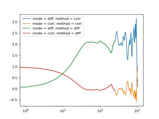
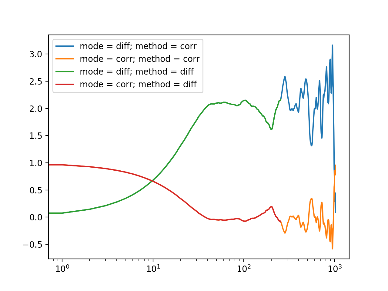
Fig. 18 Auto-correlation performed with different calculation methods and normalized with different modes are all equivalent representations. (Source code, png, hires.png, pdf)

Binning & Error

Here we will briefly cover the binning modes and the error of the obtained correlation functions with different binning options. In multiple-tau algorithm the binning option defines how the data in each of the levels is calculated. With binning=1 (multitau.BINNING_MEAN) average two measurements when adding to the next level of the correlator. With binning=0 (multitau.BINNING_FIRST) use only the first value when adding to the next level. With binning=2 (multitau.BINNING_CHOOSE) randomly select value when adding to the next level of the correlator. Default value is binning=1 (multitau.BINNING_MEAN), except if method=’diff’, where binning=0 (multitau.BINNING_FIRST) is default, as here the averaging is not supported.

With binning=1 the statistical noise is significantly lower than with the other two binning options, at the cost of some slight systematic error introduced by the averaging. The size of this error is small if level_size is large enough. binning=2 (multitau.BINNING_CHOOSE) is considered experimental. The random selection is expected to remove oscillations in correlation function because of signal beating in some experiments (particle flow with oscillating correlations). Note that you should generally use binning=1 (multitau.BINNING_MEAN), except in case you use method=’diff’, which does not support averaging.

Using binning=0 completely removes the systematic error at the cost of increasing the statistical error. This is demonstrated in the example below. Please read the source code for details.

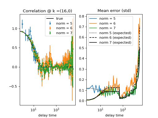
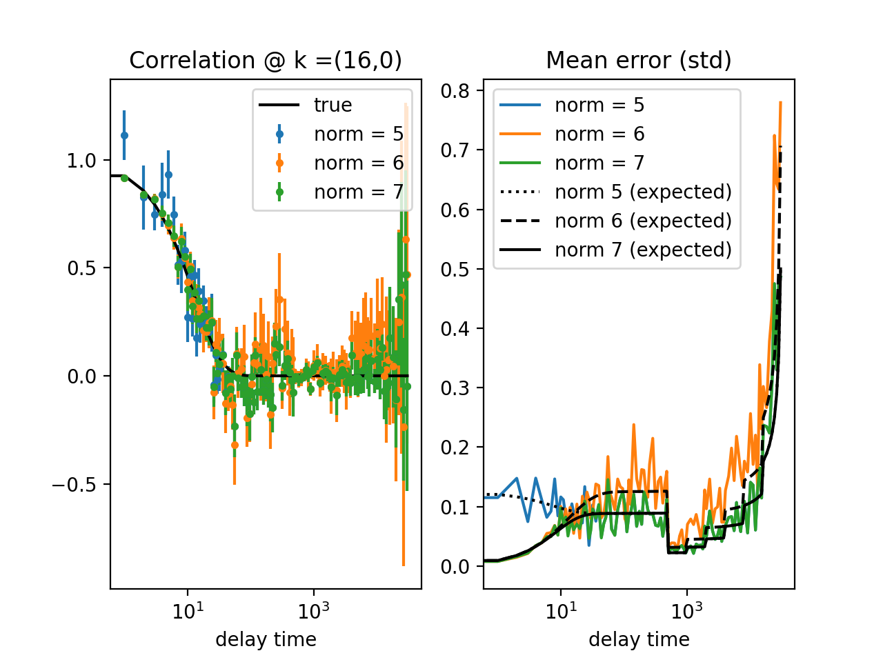
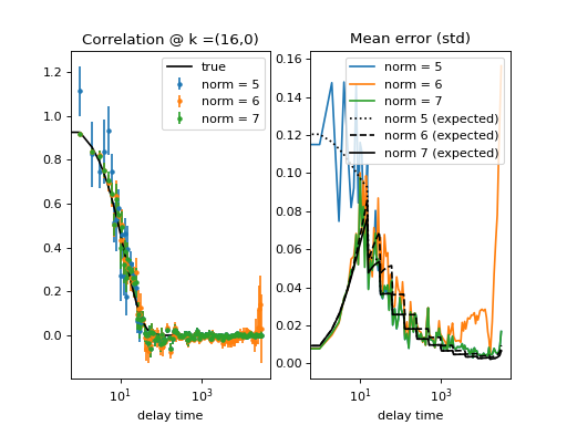
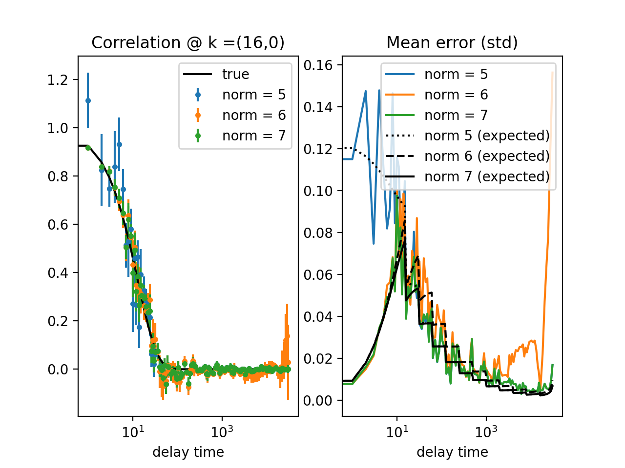
Fig. 19 (png, hires.png, pdf) Calculation of the standard deviation of data points. Several runs of the same experiment were performed to obtain different realizations of the calculated correlation function. Top graph is for binning = 0, lower graph is for binning = 1 in both the calculation and data merging steps. See source code for details. When the decay of the correlation function is shorter than the effective period of the triggering of the irregular time-spaced correlation calculation, the collected datapoint are statistically independent and there is a simple error-model estimator (in black) that compares well with the actual data point error (in color). (Source code)

Fig. 20 (png, hires.png, pdf) Calculation of the standard deviation of data points. Several runs of the same experiment were performed to obtain different realizations of the calculated correlation function. Top graph is for binning = 0, lower graph is for binning = 1 in both the calculation and data merging steps. See source code for details. When the decay of the correlation function is shorter than the effective period of the triggering of the irregular time-spaced correlation calculation, the collected datapoint are statistically independent and there is a simple error-model estimator (in black) that compares well with the actual data point error (in color). (Source code)

Live video

In Cross-DDM experiments it is important that cameras are properly aligned and in focus. For this you need a live video preview. There are some helper functions for visualizing frame difference, fft or plain video. For this to work you really should be using cv2 or pyqtgraph, because these libraries are better suited for real-time visualization of videos, so you should first install these. If you have them installed, take the library of choice:

>>> previous = cddm.conf.set_showlib("cv2")
>>> previous = cddm.conf.set_showlib("pyqtgraph") #or

Now, we have a dual-frame video object from our previous example, so we can prepare new video iterator that will show the video (first camera), difference, and fft (second camera)

>>> from cddm.video import show_video, show_diff, show_fft
>>> video = show_video(video, id = 0) #first camera
>>> video = show_diff(video)
>>> video = show_fft(video, id = 1) #second camera

The above show functions prepare the plotting library, but do not yet draw to it, you have to call video.play() with the desired frame rate to create a new video iterator that draws images when iterating over it

>>> video = play(video, fps = 100)

Now to show this video iterator, just load it into memory, or iterate over the frames:

>>> for frames in video:
...    pass

Note

The fps option should be set to the desired fps of your camera acquisition. Images are drawn only if the resources to perform the visualization are available (drawing is fast enough). Otherwise the frames will not be drawn. The iterator will go through all data, but frames will only be displayed if there are enough resources to complete this task.

Data masking

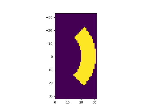
Sometimes, you may not want to compute the correlation function for the rectangular k-space area defined by the kimax and kjmax parameters of the fft.rfft2() function, but you may want to focus the analysis on a subset of k-values. This can be done most easily by video masking. You must define a boolean array with ones defined at k-indices where the correlation function needs to be calculated. For instance, to calculate data only along a given sector of k-values, you can build the mask with:

>>> from cddm.map import k_indexmap, plot_indexmap
>>> kmap = k_indexmap(63,32, angle = 0, sector = 90)
>>> m = (kmap >= 20) & (kmap <= 30)
>>> plot_indexmap(m)
>>> plt.show()

Fig. 21 Example FFT mask array. (Source code, png, hires.png, pdf)

Here we have constructed the k-mask with a shape of (63,32) because this is the shape of the fft data array. Of course you can construct any valid boolean mask that defines the selected k-values of your input data. To apply this mask to the input data there are two options. You can mask the data with video.mask()

>>> from cddm.video import mask
>>> fft_masked = mask(fft, mask = m)

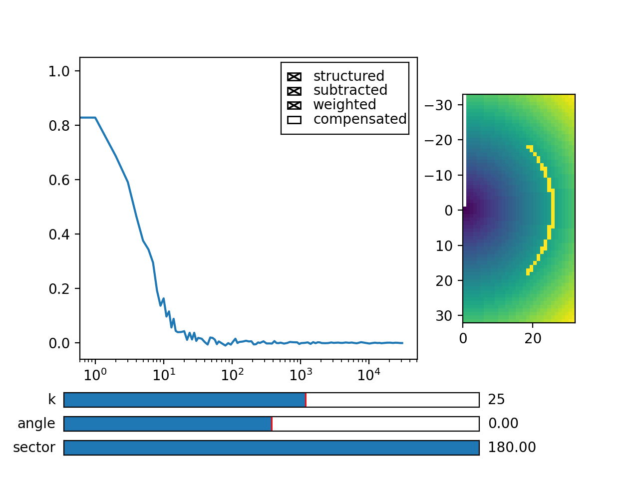
If you want to use the viewer, you will have to provide the mask to the viewer as well

>>> viewer = MultitauViewer(scale = True, mask = m, shape = (512,512))
>>> viewer.k = 25 #central k
>>> viewer.sector = 180 #average over all phi space.

Note

For rectangular-shaped video frames, the unit size in k-space is identical in both dimensions, and you do not need to provide the shape argument, however, for non-rectangular data, the step size in k-space is not identical. The shape argument is used to calculate unit steps for proper k-visualization and averaging.

Now you can calculate the masked fft data.

>>> data, bg, var = iccorr_multi(fft_masked, t1, t2, period = 32,
...   level_size = 16, viewer = viewer)

Fig. 22 Because we have computed data over a sector of width 90 degrees, we average only over the computed data values (marked with yellow dots in graph right). (Source code, png, hires.png, pdf)

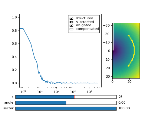
If you are working with the iterative algorithm, instead of fft masking of the input data, you can provide the mask parameter to the compute functions. E.g.:

>>> data, bg, var = iccorr_multi(fft, t1, t2, period = 32, mask = m,
...   level_size = 16)

Note that here we use the original fft (unmasked) data. The actual output data in this case is a complete-sized array, with np.nan values where the computation mask was non-positive. Regardless of the approach used, if you are doing k-selection, you have to provide the mask parameter as well:

>>> fast, slow = normalize_multi(data, bg, var, scale = True)
>>> x,y = log_merge(fast, slow)
>>> k_data = k_select(y, angle = 0, sector = 30, shape = (512,512), mask = m)

That is it, we have shown almost all features of the package. You can learn about some more specific use cases by browsing and reading the rest of the examples in the source. Also read the Configuration & Tips for running options and tips.